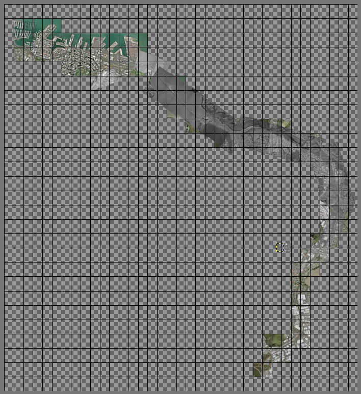
So I have been trialling the alternative overlay method with more files and have decided to redo all the mosaics for Auckland so far. This is a few days’ work but as there are already some issues with accuracy in some of the more hilly areas or where the embankment is raised, it is going to bring improvements. However, file size savings are harder to nail down, and in general I think I am not seeing consistent meaningful reductions across a range of files. What I have arrived at to maximise file size saving, is to do a bulk crop to 50% of the original size, and then custom crop each layer to just the amount that is needed, that will vary from layer to layer depending on what is needed to align with the surrounding terrain (roads etc) to get smaller still. Currently this technique is being used on a big mosaic project, Auckland-Westfield NIMT, which covers 14 km of corridor and has around 180 layers. OK so there I broke my rule, by cropping the historical layers so much we can save a lot on disk usage and have more of them, but I am still having to test the water with so many layers in this project using just a small part of a very large canvas of 35 gigapixels which is probably the biggest canvas ever, as well, and that aggressive cropping is necessary to ensure the file size doesn’t balloon unmanageably. Here’s a screenshot of the canvas, with all the base tiles in place. The Port of Auckland can be seen upper left. This corridor was opened in 1930, the original route of the NIMT being the western line that became the North Auckland Line and Newmarket Branch dating from 1873.

This post outlines the last stage in this georeferencing process, which is to extract tiles from the mosaic project that can be imported into the GIS and used to produce historical maps that are accurate in positioning of features compared to present day maps. This being, of course, the major point of the whole exercise. There are some important considerations, the first being whether to use the same tile size, 4800×7200 in this case, as the base imagery, or combine a number of tile spaces into a larger sized tile. I tend to go for this latter option since it is just less work in extraction. The important issue here is to use the grid to get the top left corner to be the same as an existing background tile so that I can copy the coordinates from that existing tile when I need to make the sidecar files for the mosaic tiles. Sometimes there isn’t one available and we will need to calculate the coordinates off the nearest available tile and here using EPSG:3857 with its coordinates expressed in metres we get a distinct advantage over a CRS that has its coordinates expressed in degrees because all you have to do, knowing the pixel resolution in metres, is make a simple calculation. In this case with this layer, at 0.1 metre pixel resolution of the base tile, each of those tiles covers an area that is 480 metres wide and 720 metres high. It then is straighforward to alter the top/left coordinates in the world file using these numbers.
The second consideration is how to name the new tiles. I always base my names on the original base tiles with a prefix. If the base tile gets scaled up or down, I also put a suffix on the original name to show that it has been resized. Let’s say I have a base tile 93Y35-92S5Z that has been scaled double in each direction, I will have renamed it 93Y35x2-92S5Zx2. Then the prefix will be a single letter representing the station and followed by four digits representing the year. Then with a tile area that covers multiple original tiles I am going to use a filename that shows the first tile and the last tile in the range covered. So here is what my large mosaic tile’s filename might look like:
X1984-93Y35x2-92S5Zx2+93Y3Bx2-92S63x2.jpg
So in there we have station X in 1984, and then the range using layers that have been scaled up by 2 a side. Note the use of the + character which may not be permitted in Windows, this file name is legal in Linux which I use and which has far fewer filename letter restrictions than Windows. This is just an example – I don’t know if I can cover all that large area in one file, as Gimp does have an export size limit, it may not be an efficient space to cover in one single file, and in this example we are actually not scaling 0.1 metre tiles up by two times anyway.
My sidecar files are .jgw, .xml and .jpg.aux.xml and they all have to be given the same base name with the correct extension and we just copy the ones from the original base tile for the top left corner (93Y35-92S5Z in this example). The only change we need to make is in the jgw file – if we have scaled then the pixel resolution measurements need to be changed e.g. from 0.3 to 0.15 m. This is well described in previous posts. I described earlier in this post how I might change the top-left coordinates in the same file if I didn’t have a set of sidecar files already downloaded to match the top left base tile in the area I am covering. Other posts on this blog describe the world file format in general and what those six numbers mean.
So hopefully in this series of posts I have adequately covered how to georeference the historical aerial layers in Gimp and how to get them into the GIS. Along the way I have learned some stuff as well, which is why I like to write these articles.